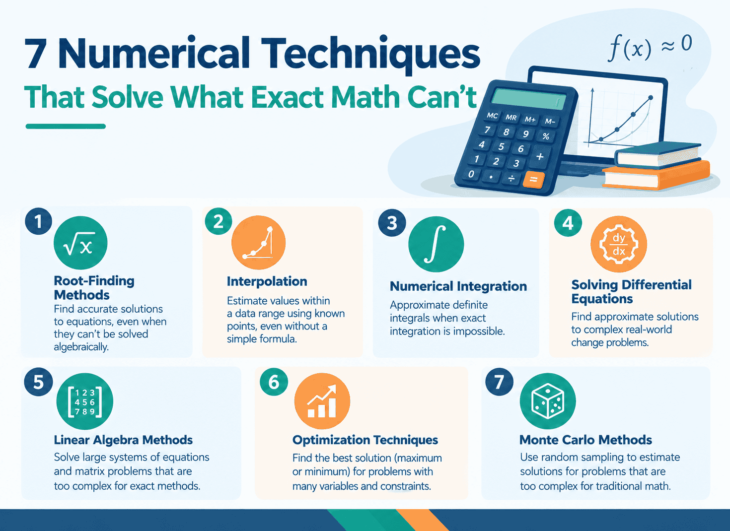
Numerical methods are step-by-step procedures that produce approximate answers to math problems when an exact formula is out of reach. Instead of solving an equation symbolically, you run an algorithm that gets closer to the answer with every step, until the error is small enough to ignore.
That one idea powers weather forecasts, bridge designs, option pricing, and the training of machine learning models. This guide covers the seven techniques you’ll meet most often, shows each one with real numbers you can check by hand, and explains how to pick the right one.
What Are Numerical Methods?
A numerical method is an algorithm that turns a hard continuous problem into a finite list of arithmetic operations. You trade a perfect answer for a good one you can actually compute.
Take the integral of e^(−x²). No elementary formula exists for it. Take a fifth-degree polynomial equation. No general formula exists for its roots either. Real engineering problems are usually messier than both. Numerical methods handle all of them.
The field that studies these algorithms is called numerical analysis. It cares about three questions:
- Accuracy: how close is the answer to the true value?
- Convergence: does the method actually get closer as you refine it?
- Cost: how many operations does it take?
Why Errors Are Part of the Deal
Every numerical answer carries error. Two sources matter most.
Truncation error comes from the method itself. When you replace a curve with straight line segments, or an infinite series with its first few terms, you throw something away.
Round-off error comes from the computer. Machines store numbers with finite precision, so tiny rounding slips pile up over millions of operations.
Good numerical work keeps both under control. A method is stable if small errors stay small instead of snowballing. You’ll see that word again below.
1. Root-Finding Methods
Root-finding answers one question: for which x does f(x) = 0?
We’ll solve x³ − x − 2 = 0. Since f(1) = −2 and f(2) = 4, a root sits between 1 and 2.
Bisection method
Bisection cuts the interval in half, checks which half still contains the sign change, and repeats.
| Step | Midpoint | f(midpoint) | New interval |
|---|---|---|---|
| 1 | 1.5 | −0.125 | [1.5, 2] |
| 2 | 1.75 | 1.609 | [1.5, 1.75] |
| 3 | 1.625 | 0.666 | [1.5, 1.625] |
| 4 | 1.5625 | 0.252 | [1.5, 1.5625] |
| 5 | 1.53125 | 0.059 | [1.5, 1.53125] |
After five steps the root is trapped in an interval of width 0.03. The true root is about 1.52138.
Bisection is slow but safe. It always works if the function is continuous and the signs differ at the ends.
Newton-Raphson method
Newton’s method uses the slope. From a guess x, the next guess is x − f(x)/f′(x). Here f′(x) = 3x² − 1.
- Start at x₀ = 1.5. Then f = −0.125 and f′ = 5.75, so x₁ = 1.52174.
- At x₁, f ≈ 0.00214 and f′ ≈ 5.947, so x₂ = 1.52138.
Two steps got us to five correct digits. Bisection needed far more.
The catch: Newton’s method can fail. If f′(x) is close to zero, the next guess shoots off somewhere wild. A bad starting point can also send it to the wrong root.
A practical habit: many solvers start with bisection to narrow the range, then switch to Newton or the secant method for the final speed.
2. Numerical Integration
When you can’t integrate a function exactly, you add up areas of simple shapes instead.
We’ll estimate the integral of sin(x) from 0 to π. The exact answer is 2. Use four slices, so h = π/4.
Trapezoidal rule treats each slice as a trapezoid:
T = h × (0/2 + 0.7071 + 1 + 0.7071 + 0/2) ≈ 1.896
That’s about 5% low.
Simpson’s rule fits a small parabola across each pair of slices:
S = (h/3) × (0 + 4 × 0.7071 + 2 × 1 + 4 × 0.7071 + 0) ≈ 2.0046
That’s off by roughly 0.2%, using the same four slices. Simpson’s rule earns its reputation: for smooth functions, it gets much more accuracy per function evaluation.
3. Numerical Differentiation
Computers can’t take limits, so derivatives become differences between nearby function values.
Estimate the slope of f(x) = x² at x = 3. The true value is 6. Use h = 0.1.
- Forward difference: (f(3.1) − f(3)) / 0.1 = (9.61 − 9) / 0.1 = 6.1
- Central difference: (f(3.1) − f(2.9)) / 0.2 = (9.61 − 8.41) / 0.2 = 6.0
Central differences are more accurate because the errors on each side cancel. They cost one extra function evaluation.
Watch the step size. Make h too large and truncation error grows. Make it too tiny and round-off error takes over, because you’re subtracting two nearly identical numbers. There’s a sweet spot in between.
4. Solving Linear Systems
Large systems of equations sit behind structural analysis, circuit simulation, and data fitting. Two families of methods handle them.
Direct methods such as Gaussian elimination and LU decomposition reach the answer in a fixed number of steps. They work well for small and medium systems.
Iterative methods such as Jacobi and Gauss-Seidel start with a guess and improve it. They shine on huge, sparse systems where direct methods eat too much memory.
Here’s Gauss-Seidel on a tiny system:
4x − y = 3
−x + 4y = 5
Start at (0, 0), then update x using the latest y, and y using the latest x.
| Iteration | x | y |
|---|---|---|
| 1 | 0.7500 | 1.4375 |
| 2 | 1.1094 | 1.5273 |
| 3 | 1.1318 | 1.5330 |
The exact solution is x = 1.1333, y = 1.5333. Each pass closes the gap.
One warning: iterative methods only converge under certain conditions. Diagonally dominant systems, like the one above, are the safe case.
5. Interpolation and Curve Fitting
These two ideas sound alike but do different jobs.
Interpolation builds a curve that passes through every data point exactly. Use it when your data is trustworthy and you need values in between. Lagrange polynomials, Newton’s divided differences, and splines are the standard tools.
Curve fitting (approximation) builds a curve that follows the overall trend without hitting every point. Least-squares regression is the classic example. Use it when your data is noisy.
Splines usually beat a single high-degree polynomial. High-degree polynomials can swing wildly between points, a problem known as Runge’s phenomenon. Splines stitch together low-degree pieces and stay well behaved.
6. Ordinary Differential Equations
Differential equations describe change: a cooling cup of coffee, a swinging pendulum, a growing population. Most real ones have no closed-form solution.
We’ll test two methods on dy/dx = y with y(0) = 1. The exact solution is y = eˣ, so y(1) = e ≈ 2.71828.
Euler’s method takes small straight steps along the slope.
| Step size | Result for y(1) | Error |
|---|---|---|
| h = 0.1 | 2.5937 | 4.6% |
| h = 0.05 | 2.6533 | 2.4% |
| h = 0.01 | 2.7048 | 0.5% |
Halving the step size roughly halves the error. That’s reliable, but costly.
Fourth-order Runge-Kutta (RK4) samples the slope four times per step and blends them. With h = 0.1, it gives 2.71828, which matches the exact value to five decimal places. Ten steps. Same step size Euler used to land 4.6% off.
This is why RK4 became the workhorse for general-purpose ODE solving. Modern software goes further with adaptive step sizes, taking small steps where the solution changes fast and large steps where it’s calm.
7. Partial Differential Equations
Partial differential equations (PDEs) describe things that change across space and time: heat flowing through metal, air moving over a wing, waves crossing water.
Three families dominate:
- Finite difference methods lay a grid over the problem and replace derivatives with differences. Simple and fast to code.
- Finite element methods break complex shapes into small elements. Standard in structural engineering, where geometry gets irregular.
- Finite volume methods track the flow of quantities between cells. Popular in fluid dynamics because they conserve mass and energy by design.
PDE solvers combine every idea above: grids, differences, linear system solves, and careful error control.
Which Method Should You Use?
| Problem | Reliable choice | Faster choice |
|---|---|---|
| Find a root | Bisection | Newton or secant |
| Area under a curve | Trapezoidal rule | Simpson’s rule |
| Derivative from data | Central difference | Higher-order stencils |
| Small linear system | Gaussian elimination | LU decomposition |
| Huge sparse linear system | Gauss-Seidel | Conjugate gradient |
| Initial value problem | Euler (for learning) | RK4 or adaptive RK |
| Noisy data | Least squares | Regularized fitting |
| Heat, wave, flow | Finite difference | Finite element or volume |
Three questions help you choose:
- How smooth is the problem? Smooth problems reward higher-order methods. Jagged ones don’t.
- How big is it? Size decides between direct and iterative approaches.
- What matters more, safety or speed? Bisection never fails. Newton usually wins, but not always.
Where Numerical Methods Show Up
- Engineering: stress analysis in bridges and aircraft, heat transfer in engines, fluid flow in pipes.
- Weather and climate: forecasts come from solving PDEs on a global grid.
- Finance: options without closed-form prices get valued with finite difference schemes and Monte Carlo simulation.
- Machine learning: training a model is numerical optimization. Gradient descent is a numerical method.
- Computer graphics: lighting, physics engines, and animation all lean on numerical approximation.
- Medicine: imaging reconstruction and blood-flow simulation rely on the same toolkit.
How to Start Learning Numerical Methods
Don’t begin with theory alone. Pick one problem, solve it by hand with two methods, then code both.
- Learn error types first. Everything else depends on them.
- Implement bisection and Newton in a few lines of Python.
- Move on to Simpson’s rule, then Euler and RK4.
- Use a library once you understand the basics. NumPy and SciPy cover almost everything in this article, and MATLAB and Julia are strong alternatives.
Check your code against a problem with a known answer, as we did with sin(x) and eˣ above. If your method can’t reproduce a known result, it won’t be trustworthy on an unknown one.
Frequently Asked Questions
What are numerical methods in simple terms?
They’re algorithms that find approximate answers to math problems when exact answers are impractical or impossible. You repeat a simple calculation many times, and each pass gets closer to the true value.
What is the difference between numerical methods and numerical analysis?
Numerical methods are the individual algorithms. Numerical analysis is the field that designs them and studies their accuracy, stability, and cost.
Why do we need numerical methods if we have calculus?
Calculus gives exact answers only for problems with tidy formulas. Most real-world equations don’t have one. Numerical methods fill that gap.
Are numerical methods always approximate?
Yes. Even so, you can usually push the error below any tolerance you choose, as long as you accept more computation time.
Which numerical method is best?
None wins everywhere. Bisection is the safest root finder, Newton is the fastest on well-behaved problems, and Simpson’s rule beats the trapezoidal rule on smooth curves. Match the method to the problem.
What programming languages are used for numerical methods?
Python (with NumPy and SciPy), MATLAB, Julia, C++, and Fortran. Python suits learning and prototyping. Fortran and C++ still run many large scientific simulations.
Key Takeaways
- Numerical methods trade exactness for answers you can actually compute.
- Error comes from two places: the method (truncation) and the machine (round-off).
- Newton’s method converges fast, bisection converges safely, and good solvers often use both.
- Simpson’s rule and RK4 deliver big accuracy gains over their simpler cousins at modest extra cost.
- Always test a method against a problem with a known answer before trusting it on a new one.